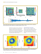
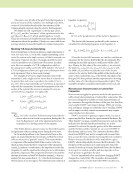
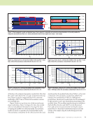
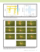
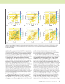
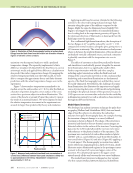
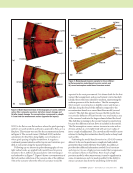
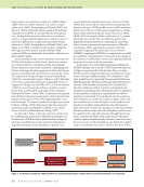
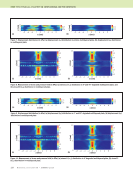
88 M A T E R I A L S E V A L U A T I O N • J A N U A R Y 2 0 2 0 ME TECHNICAL PAPER w angle-beam pulse-echo ultrasonic inspection In other words, the images represent only half of the path the sound travels. For the case of the half-skip, half of the distance “inside the PMC” is the point where the wave arrives at the backwall of the panel. This is because the half-skip signal path length, as it travels to the backwall directly, is the same as the path length that reflects from SDH2 and down to the bottom surface (Figure 2b). Note, the total path and time of flight are complicated by the fact that the oblique path in water is longer for one side of the transducer and shorter for the other side, as shown in Figures 5b and 5e. The full-skip half-path length is easier to identify since the full-skip travels to the backwall, reflects, travels to SDH2, scatters, and travels back to the backwall and reflects back to the transducer. From this, it is clear that the half-path length of the full-skip signal occurs when the wave interacts with SDH2. The expected wave posi- tions and times of flight for the half-skip (B-D path described previously) at 5.88 μs and full-skip (B-D-B path also described previously) at 6.5 μs agree with the wave propagation results in the wave maps shown in Figure 7. Side-Drilled Hole Model Benchmarking with Experimental Data The SA-FDTD and FEM models agree well with experiments for SDH1, while there is increased variation in the results for SDH2. The SA-FDTD model, in general, shows more devia- tion from the experimental results than the FEM solution, but it is sufficient as a means to interpret the experimental results. Differences among the SA-FDTD model, FEM model, and the experiments account for these deviations. The SA-FDTD model makes a number of assumptions, such as using a semi- analytical beam model (with Auld’s reciprocity theorem), nominal material properties, ideal surface conditions, and not accounting for near-field effects of the transducer. A unique aspect to this problem is how the focused beam will behave inside the specimen. Focused transducers are designed to focus a beam in normal incidence. When operated obliquely, there is less focusing and side lobes can be present, shown on either side of the main pulse in Figure 7. These side lobes have their own distinct propagation paths and can interact with the main pulse. When the SA-FDTD results are contrasted with the expected variation in the experimental values due to these factors, the differences seen are reason- able. The FEM model makes fewer assumptions, and it is in general closer to the experimental results as expected. This is due to the FEM model being able to account for the trans- ducer characteristics and the near-field wave propagation more accurately than the SA-FDTD model. Deviations between FEM and the experiments illustrate that the assump- tions made in the FEM model, such as transducer parameters that are usually more than sufficient for normal-incidence inspections in homogeneous materials, yield significant differ- ences to the experiments. Oblique ultrasound, layered mate- rials, and anisotropic materials are all challenging to model and inspect alone. Combining them all into one inspection and being able to interpret the results is an exceptional challenge. In Figure 8, the SA-FDTD model B-scan results for the SDH test specimen are compared with results from the FEM model and experiments. The SA-FDTD model results show good qualitative agreement with FEM and the experimental results. The B-scan images are annotated to show the location of the direct reflection from the SDH, the full-skip (Figures 5a and 5d), and the half-skip (Figures 5b and 5e signals). In the cases of the SA-FDTD and FEM models, skip locations were determined from wave maps as discussed in the “Models for Complex-Signal Interpretation” section of this paper. For the experimental data, the backwall skip locations were identified by locating secondary signal peaks to the left of and later in time relative to the peak direct reflection from the SDH, with guidance from the simulations. Ray tracing was also used to estimate the TOF and location of the expected direct and full- skip signals, and these estimates correlated well with the SA-FDTD results. The horizontal signal bands in TOF in the SA-FDTD B-scans beginning at approximately 9.5 μs and 11.3 μs are the result of using a focused transducer at an oblique angle very close to a specimen. The cases presented here are very close to the face of a focused transducer. Near the face of a focused transducer there are side lobes present that are created by the lens. The effect of these side lobes dissipates rapidly with distance, and the side lobes are rarely seen when a focused transducer is used for normal-incidence inspections. The effect of the focused transducer side lobes is seen in this example because of the short focal length (11.4 mm), very short water path length (7 mm), and the transducer being used in an angle-beam configuration. When operated very close to a surface at an oblique angle, a portion of the side of the focused transducer farthest from the surface remains normal to the surface, as seen in Figure 5. This combination of effects allows a normal incident wave front to still exist, which can be called the normal beam component (NBC). The horizontal band at approximately 9.7 μs corre- sponds to the longitudinal time of flight from the transducer to the front surface of the PMC, and the horizontal band at approximately 11.3 μs corresponds to the signal from the back surface of the composite. This was verified by a ray-trace calculation and wave-map analysis. These NBC signals are present in FEM (~9 μs and ~11 μs) and experimental data (~9 μs and ~10.5 μs) as well, but they are less prominent. There are several additional signals present that can confound data interpretation, but they can be identified in wave-map analysis. The strong return signals occurring earlier in time and shifted to the right of the direct signal are related to the NBC interactions with the SDH and the top surface. The strong return signals near the direct signal, but slightly later in time and to the left, are the NSI and FSI signals discussed in the “Models” section of this paper and shown in Figures 5c and 5f. The horizontal band of strong signal at approximately 16 to 17 μs in the FEM data (Figures 8c and 8d) is attributed to numerical noise (grid effects, discretiza- tion, or other numerical errors in the model result in spurious

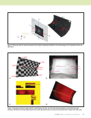
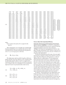
J A N U A R Y 2 0 2 0 • M A T E R I A L S E V A L U A T I O N 89 signals), as this is not present in the SA-FDTD or experimental observations, and the origin could not be accurately determined in the wave-map analysis either. The high-amplitude signals in the experimental data for SDH1 (Figure 8e at 26 mm, 15 μs) and SDH2 (Figure 8f at 77 mm, 14 μs) are possibly the result of a side-lobe skip, but additional analysis is required to confirm this. There are other signals present as well, but these consist of multiple-reflection interactions that are exception- ally difficult to deconvolve even with wave-map analysis. The interpretation of the FEM and experimental responses is further confounded by additional transducer near-field effects, which is a result of the transducer-to-sample water-path distance being only slightly longer than the expected near-field distance, which is not considered when using a semianalytical solution such as SA-FDTD. Additionally, beam effects from operating a focused transducer in oblique incidence in a layered anisotropic material further compound the challenges already present in the interpretation. A quantitative comparison of the results for direct, half-, and full-skip signals is presented in Table 1. It should be noted that for the case of the experiment, the lateral position of the peak direct-reflection signal relative to the SDHs could not be determined with certainty and is not reported. However, in the models it is challenging, but it is possible, to locate the reflection position relative to the SDH. The SA-FDTD and FEM models agree with each other and to the experimental results except for some notable differ- ences that will be discussed here in greater detail. Both the SA-FDTD solution and the FEM solution predict a later arrival time for the full-skip from SDH1 and an earlier arrival time for SDH2 than is seen in the experimental results. The position of the full-skip predicted by SA-FDTD is consistently nearer to the SDH than is observed in experiments. Overall, the FEM solution provides predictions that are closer in time and position to what is observed in experiments for SDH1. Conversely, SA-FDTD results in general better correlate to experimental results for SDH2. This is unexpected and addi- tional testing is required to determine under what conditions SA-FDTD modeling produces results that are a better match to experiments than FEM. The most likely source of these differences is attributed to the use of a semianalytical beam model (with Auld’s reciprocity theorem) in the SA-FDTD model versus solving the probe model numerically in the FEM model. Given the sharp focus of the transducer, oblique 18 16 2 4 6 8 10 12 14 12 10 8 4 3.5 3 2.5 2 1.5 1 0.5 0 x (mm) 18 16 18 20 22 24 26 28 14 12 10 8 4 3.5 3 2.5 2 1.5 1 0.5 0 x (mm) 18 16 2 4 6 8 10 122 14 12 10 8 0.033 0.025 0.02 0.0155 0.01 0.005 0 x (mm) 18 16 18 20 22 24 26 28 14 12 10 8 x (mm) 0.03 0.0255 0.02 0.0155 0.01 0.005 0 18 16 24 26 28 30 32 34 14 12 10 8 80 70 60 50 40 30 20 10 0 x (mm) 18 16 75 77 79 81 83 855 14 12 10 8 x (mm)m) 800 700 600 50 400 300 200 10 0 1 0 m) 18 8 0 2 12 10 3 5 2 1 0 0 1 1 0 8 4 1 m) 0 0 0 0 0. 1 0 5 0 12 10 80 70 60 50 40 30 20 m) 5 9 1 1 8 7 6 4 3 2 SDH1 direct SDH2 direct SDH1 full skip SDH2 full skip SDH2 full skip SDH2 full skip SDH1 full skip SDH1 half skip SDH2 half skip SDH2 half skip SDH2 half skip SDH1 half skip SDH1 direct SDH1 direct SDH1 half skip SDH1 full skip SDH2 direct SDH2 direct Figure 8. B-scan images of the polymer matrix composite with side-drilled holes: (a) SA-FDTD model for SDH1 (b) SA-FDTD model for SDH2 (c) FEM for SDH1 (d) FEM for SDH2 and experiments with location of direct reflection and full-skip signals marked by parallelograms for (e) SDH1 and (f) SDH2. (a) (d) (c) (b) (e) (f) Amplitude (a.u.) Amplitude (a.u.) Amplitude (a.u.) Amplitude (a.u.) Amplitude (a.u.) Amplitude (a.u.) (a . A m A m (a . Time (μs) Time (μs) Time Time (μs) Time (μs) Time ((μs) ) ((μs) )