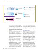
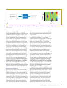
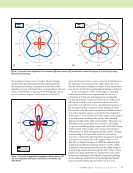
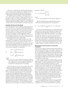
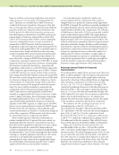
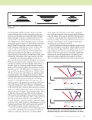
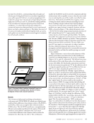
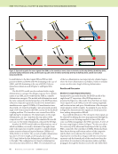
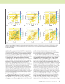
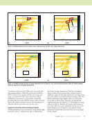
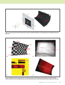
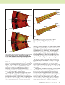
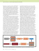
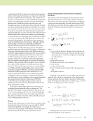
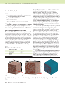
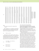
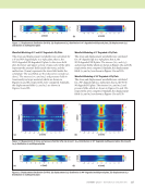
112 M A T E R I A L S E V A L U A T I O N • J A N U A R Y 2 0 2 0 (16) where “Zeros” indicate the matrix of 0s as required in the equation. After obtaining the source strengths, the wavefield inside fluid and solid half space was computed. The pressure field inside the fluid was calculated using the following equation, where F is a set of target points in the fluid. (17) The displacement and stress fields (together called wave- fields) inside the anisotropic half space were calculated using the following equations where m is the set of target points distributed inside the solid where the wavefields are intended to be computed. The stress and displacement wavefields from Equations 8 and 10 are presented in the results section. (18) (19) Process to Boost the Computational Efficiency Symmetry informed sequential mapping of anisotropic Green’s function (SISMAG). To boost the computational efficiency, two propositions based on the symmetry informed sequential mapping of anisotropic Green’s function (SISMAG) were introduced and implemented for the 1-ply plate (Shrestha and Banerjee 2018). However, in the case of a multilayered plate, three propositions based on SISMAG were introduced and implemented. The first two propositions are the same as the ones imple- mented in the 1-ply plate and discussed in detail in a previous paper (Shrestha and Banerjee 2018) and hence can be also employed here in a similar manner. The first proposition dictates that the Green’s function at a target point due to a unit load acting on the source point is always the same if the direction cosine of the line joining the source–target combi- nation is constant. The second proposition is the symmetry of the Green’s function at the bottom and top interfaces. This is true only if the material property in between two interfaces is constant and the material is homogeneous. Hence, with the implementation of this argument, the Green’s function needs to be calculated at only one interface and it can be sequen- tially and symmetrically mapped on the other interface. In addition, a third proposition is also implemented. The third proposition is the identicality of the Green’s function for the layer with the same material properties as shown in Figure 5. Similar to the second proposition, it is also true only if the material properties between the two interfaces, or the lamina layers, are constant, and the material is homogeneous. PR P A P AI F FS S FI = + U1 UAX A U2 UAY A U UAZ A 3m m mI I m mI I* mI I* * * * * = = = S AI* S A S A 33 31 32 m mI m mI I* m mI I* * * * = L33 = L31 = L32 ME TECHNICAL PAPER w computational nde for composites

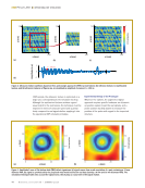
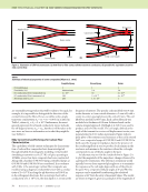
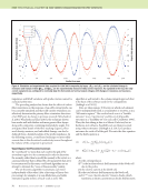
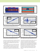
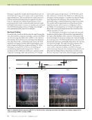
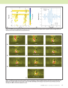
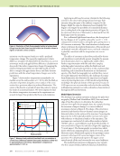
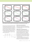
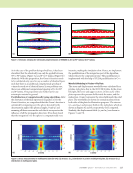
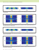
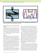
J A N U A R Y 2 0 2 0 • M A T E R I A L S E V A L U A T I O N 113 As in the case of the problem being solved here, it has been elucidated that the identicality can only be applied between 90° to 90° lamina (Figure 5a) and 0° to 0° lamina (Figure 5b) distinctly. With this proposition, the Green’s function needs to be calculated only once for any n number of identical layers such that there is an additional computational speedup of n times for each set of identical layers. In our problem case, there is an additional computational speedup of 2× for 90° and 0° lamina. This proposition also holds true for any anisotropic material in general. Parallelization of computationally taxing algorithms. After the derivation of the final expression (Equation 1) for the Green’s function, we comprehend that the Green’s function is calculated by integrating over the sphere denoted by the discretization angles (the spherical angles, q and j) and summing all three wave modes such that it incorporates the influence of all the propagation direction. It has been found that the integration over the sphere is computationally very intensive, making the simulation slow. Hence, we implement the parallelization of the integration part of the algorithm, which reduces the computation time. The parallelization is implemented with the help of CUDA parallelization in C++. Wavefield Modeling in Pristine 4-Ply Plate The stress and displacement wavefields were calculated for a pristine 4-ply plate that is, the 90/0/90/0 plate. In the stress field plot, the lower and upper sections (5 mm each) of the plots represent the pressure fields inside the water, and the midsection (3 mm) represents the stress field inside the solid plate. The wavefields are shown for normal incidence from both sides of the plate for illustration purposes. The stresses (s11 and s33) and pressure fields in the 4-ply plate, which are shown in Figures 6a and 6b, respectively, were computed. Similarly, the displacement fields (u1 and u3) are shown in Figures 7a and 7b. Figure 5. Schematic showing the identicality implementation of SISMAG in 2D: (a) 90° lamina (b) 0° lamina. (a) (b) –8 –6 –4 –2 0 0 5 8 13 2 1.5 1 0.5 2 1 2 3 4 5 1.5 1 0.5 x (mm) 2 4 6 8 –8 –6 –4 –2 0 0 5 8 13 2 1.5 1 0.5 2 2 4 1.5 1 0.5 x (mm) 2 4 6 8 Figure 6. Stress measurements in multilayered plate (in GPa): (a) stress11 (σ11) distribution in pristine multilayered plate (b) stress33 (σ33) distribution in multilayered plate. (a) (b) z (mm) z (mm)