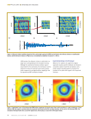
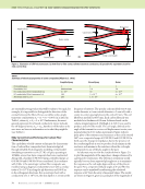
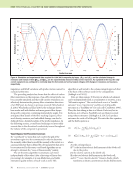
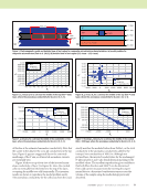
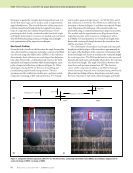
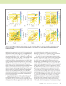
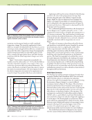
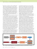
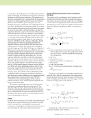
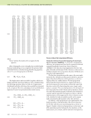
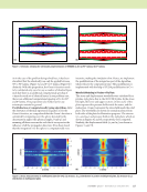
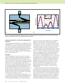
90 M A T E R I A L S E V A L U A T I O N • J A N U A R Y 2 0 2 0 angle, layered anisotropic specimen, and close proximity of the near-field to the top surface, some numerical differences are not surprising. These conditions also account for the differences between the SA-FDTD model and the experi- mental results. While the FEM model is expected to more closely repre- sent the experiments, it is also based on simplifying assump- tions to model the transducer. These assumptions are quite reasonable for normal-incidence inspections especially in homogeneous materials, but the additional complexities of a layered anisotropic material, oblique-incidence excitation, and a focused-beam transducer compound the errors. Small errors between the “ideal” beam profile used in the model and the actual transducer used in the experiments are compounded at each layer interface, which is not an issue for normal-incidence inspections. Additionally, side lobes that do not affect normal- incidence scans are now oriented in such a way that they can generate signals that interact with features of interest, and this can confound identification of the desired skip signals. Considering the complex nature of this problem, an oblique inspection of a layered-anisotropic material with a focused transducer of a specimen that is very close to the face of a focused transducer, SA-FDTD performed well, given its inherent assumptions. The effect of the focused transducer side lobes is seen in this example because on the short focal length, very short water-path length, and the transducer being used in an angle-beam configuration. It is the complexity of the problem that makes understanding the experimental results exceedingly difficult without some form of model to inform the interpretation. This is clear given the number of high-amplitude-return signals and the full-skip signal of interest not being the highest-amplitude signal. The near-field effects could be reduced or eliminated by switching to a longer focal-length transducer, but this is not expected to change the number of high-amplitude-return signals or the fact that the full-skip signal of interest is not the highest- amplitude signal. Comparison of Side-Drilled Hole and Edge-Delamination Responses After understanding the sources of the signals and verifying the basic SA-FDTD model behavior with the canonical SDH geometry, the case of a single delamination was modeled. The signals from the SDH specimen (Figure 9a) clearly show modest similarity to the delamination case (Figure 9b) when normalized to the same absolute amplitude range and plotted on different scales to show the locations of direct and skip signals. Following the same wave-map analysis discussed in the “Models for Complex-Signal Interpretation” section of this paper, the signals present in the single delamination case are identifiable. The parallel line of the signal beginning at ~9.5 μs is due to NBC, as discussed earlier. To the right of the direct signal from the delamination edge (x = 4.6–6.0 mm) is an increase in amplitude over the expected horizontal NBC signal amplitude at ~10 μs. This increase in amplitude is due to the NBC reflecting off of the top of the delamination. Simi- larly, there is an increase in amplitude of the expected hori- zontal backwall NBC signal centered at ~11.5 μs at position x = 3.5 mm due to the full-skip signal (B-D-B) from the delamination reflecting the entire signal back to the trans- ducer. Amplitude analysis shows the direct signal from the SDH is 2.6× greater than the direct signal from the delamina- tion, while the full-skip from the SDH is 3.8× greater than the full-skip signal from the delamination. The difference in signal amplitude between the SDH and delamination is attributed to the larger surface area of the SDHs resulting in more reflected energy than occurs from the waves diffracted from the edge of the delamination. ME TECHNICAL PAPER w angle-beam pulse-echo ultrasonic inspection TABLE 1 Comparison of direct and backwall skip signal locations and TOF for the side-drilled hole specimen Signal SA-FDTD FEM Experiment (position and time) SDH1 Direct: position left of SDH1 0.9 mm 0.2 mm – SDH1 Direct: TOF 10.73 μs 11.21 μs 12.06 μs SDH1 Half-Skip: position left of direct 0.4 mm 0.6 mm 0.6 mm SDH1 Half-Skip: time after SDH1 direct 1.30 μs 1.43 μs 1.15 μs SDH1 Full-Skip: position left of direct 1.6 mm 1.8 mm 1.8 mm SDH1 Full-Skip: time after SDH1 direct 1.78 μs 2.18 μs 1.65 μs SDH2 Direct: position left of SDH2 0.4 mm 0.3 mm – SDH2 Direct: TOF 9.80 μs 10.56 μs 10.78 μs SDH2 Half-Skip: position left of direct 1.6 mm 0.2 mm 2.1 mm SDH2 Half-Skip: time after SDH2 direct 2.10 μs 1.32 μs 2.09 μs SDH2 Full-Skip: position left of direct 1.8 mm 1.6 mm 3.3 mm SDH2 Full-Skip: time after SDH2 direct 3.41 μs 3.59 μs 3.77 μs

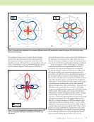
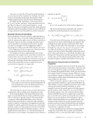
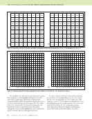
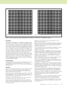
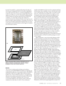
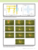
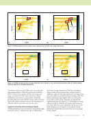
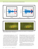
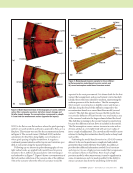
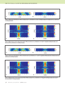
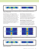
J A N U A R Y 2 0 2 0 • M A T E R I A L S E V A L U A T I O N 91 The reflection behavior of the SDH can be seen in the wave- map images in Figure 7. When the wave interacts with the SDH it continues to propagate with the same energy, but along a new direction vector. Wave interaction with the delamination tip produces an approximate cylindrically spreading diffraction field. Only the portion of the wave prop- agation that interacts with the bottom of the delamination is reflected, and this is directed away from the source. Insight into Interpreting Hidden Delamination Signals A hidden-delamination case was modeled to study whether angle- beam pulse-echo UT could detect the edge of a delamination shadowed by another delamination. The dotted rectangles in Figure 10 indicate the areas where there is a large increase in amplitude compared to the single-delamination case (Figure 10a), due to the addition of a hidden delamination (Figure 10b). The hidden-delamination signal (Figure 11b) is very clear in the A-scan taken at this location compared to the signal for the single-delamination case (Figure 11a). Following the wave-map analysis described in “Models and Complex-Signal Interpreta- tion,” these differences can be attributed to the presence to the hidden delamination (see Figure 12). It is easier to see the delamination signal in the A-scan than in the wave-map images for this example. 8 0 1 2 3 4 5 6 0 1 2 3 4 5 6 10 12 14 16 18 20 22 8 10 12 14 16 18 20 22 x (mm) x (mm) 4 3.5 3 2.5 2 1.5 1 0.5 0 1.6 1.4 1.2 1 0.8 0.6 0.4 0.2 SDH direct Delamination direct Delamination full skip SDH full skip Figure 9. SA-FDTD amplitude B-scans using the same calibration level: (a) SDH2 (b) a single delamination. (a) (b) 8 0 1 2 3 4 5 6 0 1 2 3 4 5 6 10 12 14 16 18 20 22 8 10 12 14 16 18 20 22 x (mm) x (mm) 1.6 1.4 1.2 1 0.8 0.6 0.4 0.2 1.6 1.4 1.2 1 0.8 0.6 0.4 0.2 Figure 10. SA-FDTD generated B-scans: (a) single delamination with a depth of 1 mm and (b) two delaminations where the dotted rectangle marks the signal due to the hidden delamination. (a) (b) Amplitude (a.u.) Amplitude (a.u.) Amplitude (a.u.) Amplitude (a.u.) Time (μs) Time (μs) Time (μs) Time (μs)