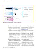
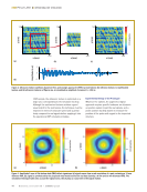
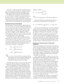
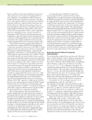
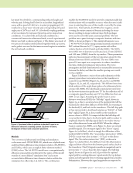
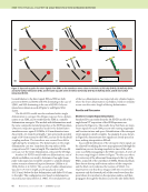
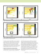
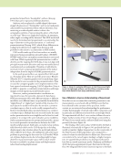
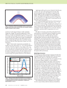
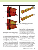
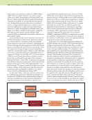
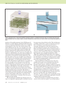
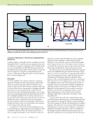
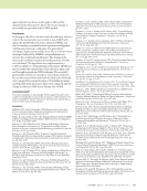
110 M A T E R I A L S E V A L U A T I O N • J A N U A R Y 2 0 2 0 interfaces of the problem geometry. In the DPSM approach (Banerjee et al. 2007 Banerjee and Kundu 2007b), the point sources are distributed behind the transducer faces (Figure 4) and distributed on either side of the interface between the solid and fluid media. A1 is the source strength vector of the point sources that are placed above the bottom fluid–solid interface and generate the additional ultrasonic field in the fluid below the plate caused by the presence of the plate. The interface is called Interface 1. A1* is the source strength vector of the sources that are distributed below the bottom fluid– solid interface and model the transmitted field in the solid plate. A2 and A2* are the source strength vectors of the point sources that have been distributed above and below the first solid–solid interface or second interface from the bottom, respectively. This interface is called Interface 2. A3 and A3* are the source strength vectors of the point sources that have been distributed above and below the second solid–solid interface or third interface from the bottom, respectively. This interface is called Interface 3. A4 and A4* are the source strength vectors of the point sources that have been distrib- uted above and below the third solid–solid interface or fourth interface from the bottom, respectively. This interface is called Interface 4. Finally, A5 and A5* are the source strength vectors of the point sources that have been distributed above and below the top fluid–solid interface, respectively. This interface is called Interface 5. Transducer faces have source strength vectors AS and AR. The total ultrasonic wavefield at any arbitrary point C in Fluid 1 is computed by superposing the contributions from all the point sources denoted by AS and A1. The total ultrasonic wavefields contributed by a various set of point sources and their contributions at any arbitrary point D inside an anisotropic solid depends on where the arbitrary point is placed. For illustration purposes, the total ultrasonic wave- fields at the arbitrary point D, which is in between Interface 3 and 4, are computed by superposing the contributions from each point sources with the Green’s function multiplied with their respective source strength denoted by A3* and A3 (Figure 4b). Similarly, the ultrasonic field can be computed for the solid points in between other interfaces as well. Finally, the total ultrasonic wavefield at any arbitrary point E in Fluid 2 is computed by superposing the contributions from all the point sources denoted by A5* and AR. After the distribution of the point sources, the source strengths of those point sources distributed over the trans- ducer and the interface are calculated by satisfying the boundary and the interface continuity conditions as required. The source strength depends on 3D force vectors for the actu- ation of the point sources. The displacements or stresses at any target point are computed with the help of source strengths and the Green’s function computed for that point. Hence, the source strengths AS, A1, A1*, A2, A2*, A3, A3*, A4, A4*, A5, A5*, and AR need to be calculated, which are unknowns. The source strengths can be calculated by solving a set of linear equations obtained after applying the boundary conditions, which are discussed below. The bottom transducer is simulated with a prescribed velocity on the circular face equal to VS0 and top transducer ME TECHNICAL PAPER w computational nde for composites R S Transducer 1 Transducer 2 A R A S A 3* A 5* A 1 A 4 C E D Solid Fluid 1 Fluid 2 Fluid 90° 0° 90° 0° Fluid z y x x-z plane x-y plane y-z plane Figure 4. Schematics (not to scale) of the wavefield computation problem in a multilayered anisotropic plate: (a) simulation setup with point sources distributed over the x-y plane however, only two orthogonal line of point sources are shown and (b) cross-sectional view along the x-z plane. (a) (b) Anisotropic plate

J A N U A R Y 2 0 2 0 • M A T E R I A L S E V A L U A T I O N 111 with VR0. At the solid–fluid Interface 1 and 5, the normal displacement and the normal stresses along the z direction should be continuous however, the shear stresses must vanish. The prescribed normal velocity VS0 and VR0 on the trans- ducer faces can be obtained by superposing the contribution of the velocity fields created by AS and AI and A5* and AR sources, respectively. By calculating the fluid domain Green’s function (Banerjee et al. 2007 Banerjee and Kundu 2007b) on the target points, the velocity equation is (5) (6) The velocity Green’s function matrices in fluid VG are written in the literature (Shrestha and Banerjee 2018) and omitted herein. On the other hand, the normal displacement at the fluid– solid interface should be continuous. The following displace- ment equations using the displacement Green’s function matrices composed of the displacement Green’s function in fluid and anisotropic solid in the z direction can be written as (7) (8) where UfZIS is the displacement Green’s function matrix for the target points at any interface I due to any point sources S spanning inside the fluid. In a similar manner, the displacement along all three direc- tions at the solid–solid interfaces should also be continuous which can be written as (9) where UADIS is the displacement Green’s function matrix along the D direction at any interface I due to any point sources S spanning inside the anisotropic solid, D = X, Y, Z, representing three directions, i = 2, 3, and 4, j = (i–1)*, k = (i)*, and l = i +1. The respective Green’s function matrices are written in the literature (Shrestha and Banerjee 2018). The compressive normal stress in the anisotropic solid and the fluid pressure at the fluid-solid interfaces should be continuous, and thus equations for stress and pressure can be written as (10) (11) Similarly, the compressive normal stresses in the anisotropic solid at the solid–solid interfaces should be continuous, and thus equations for stresses can be written as (12) where i = 2, 3, and 4, j = (i–1)*, k = (i)*, and l = i +1. Additionally, the shear stresses at the fluid–solid interface should vanish because fluid cannot take any shear stresses. Thus: (13) (14) where IJ = 31 and 32, representing the shear components. However, the shear stresses at the solid–solid interfaces should be continuous. Thus: (15) where IJ = 31 and 32, representing the shear components, i = 2, 3, and 4, j = (i–1)*, k = (i)*, l = i +1. P is the pressure Green’s function matrix in fluid and S33, S31, and S32 are the stress Green’s function matrix in the anisotropic plate for the s33, s31, and s32 stresses obtained from Equation 4, respectively. Rearranging the equations from Equation 5 to Equation 15 we get the matrix shown in Equation 16. After solving the linear algebra problem, the source strengths AI*, AS, and AI were obtained to calculate the wavefield inside the fluid and solid. VG A VG A VS0 SS S S 1 2 + = VG A VG A VR0 R RR R 5 5½ + = ½ UfZ A UfZ A UAZ A UAZ A2 S S 1 11 1 11 1 12 + = + ½ UfZ A UfZ A UAZ A UAZ A5 R R 55 5 5 54 4 55 + = + ½ ½ ½ ½ UAD A UAD A UAD A UAD Al ij j ii i ik k il + = + P A P A A A2 33 S S 1 11 1 11 1* + = [L [ L3312 + = [L [ L3355 P A P A A A5 33 R R 55* 5* 5 54* 4* A A A Al ij j ii i ik k L33 + L33 = L33 + L33il A A2 0 11* 1* 12 LIJ + LIJ = A A5 0 54* 4* 55 LIJ + LIJ = A A A Al ij j ii i ik k il LIJ + LIJ = LIJ + LIJ