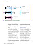
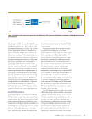
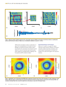
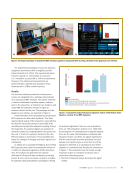
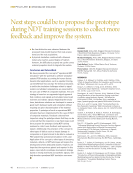
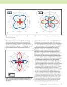
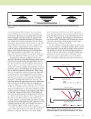
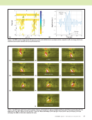
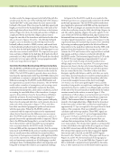
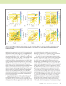
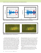
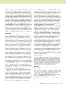
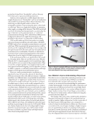
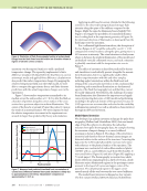
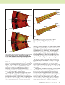
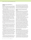
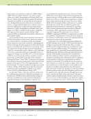
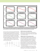
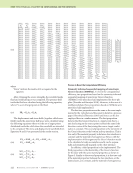
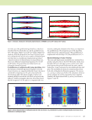
be small relative to the direct signal. FSI and NSI are both present in SDH1 and SDH2 with FSI dominating in the case of SDH1, and NSI dominating in the case of SDH2. Only one interaction is shown in each of Figure 5c and Figure 5f for clarity. The SA-FDTD model was also evaluated with a single delamination to compare the oblique response from a delami- nation to an SDH, and to verify that the SDH is a suitable delamination surrogate. The models with delaminations used the same composite material properties as the SDH specimen. Ultrasonic inspection parameters used for the delamination simulations were again 2.25 MHz, 6.35 mm diameter trans- ducer with a 11.4 mm focal length, 7 mm water path, incident angle of 18° from normal to the PMC, and air for the backwall coupling medium. The transducer was scanned from left to right during the simulations. The delamination in the single- delamination case was 1 mm from the top surface of the composite and 12.7 mm in length. The simulated B-scan did not scan over the entire delamination, only past the left edge. Another SA-FDTD model with two delaminations, one of which was hidden, was used to determine if an angle-beam pulse-echo inspection would be sensitive to a hidden delami- nation scenario referenced in prior literature (Aldrin et al. 2018 Welter et al. 2018). The second or hidden delamination was also 12.7 mm in length, and it was placed one ply (0.135 mm) below the first delamination and shifted 3.85 mm to the right. This configuration was based on delamination microstructure data (Boll et al. 1986). The simulated B-scan of the two-delamination case inspected only a limited region where the lower delamination was hidden it did not simulate a scan over the entire length of the top delamination. Results and Discussion Models for Complex-Signal Interpretation Simulated B-scan results from the SA-FDTD model of the angle-beam UT inspection of the SDH specimen are presented in Figure 6a. The results show that there are many return signals for each SDH present with varying magnitude and location in time and space. Identification of the strongest return signals is clearly complex. An example A-scan, shown in Figure 6b, demonstrates how signals are closely spaced in time, making interpretation difficult. Successful identification of the strongest return signals can be achieved by utilizing the wave maps generated through the simulation process showing snapshots in time of the ultra- sonic wavefield propagating in the PMC specimen. A series of the wave-map images is shown in Figure 7 for the case where the center ray of the ultrasound beam impacts the top of the PMC, 2 mm left of the centerline of SDH2. Horizontal black lines denote the top and bottom surfaces of the composite and the black circle indicates the location of SDH2. It is important to note that these images (with time increments) represent only the forward path of the sound wave from the point where it is incident on the specimen surface and then propagates through the thickness and to the side-drilled hole. 86 M A T E R I A L S E V A L U A T I O N • J A N U A R Y 2 0 2 0 ME TECHNICAL PAPER w angle-beam pulse-echo ultrasonic inspection Direct (D) Far-surface interaction (D-B) Direct (D) Near-surface interaction (D-B-D) Figure 5. Expected ray paths for return signals from SDH1 as the transducer moves closer to the hole: (a) full skip (B-D-B) (b) half skip (B-D) and (c) far-surface interaction (D-B) and the same ray path series for SDH2: (d) full skip (B-D-B) (e) half skip (B-D) and (f) near-surface interaction (D-B-D). (a) (d) (c) (b) (e) (f)

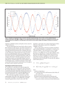
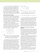
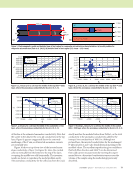
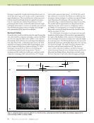
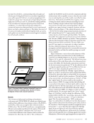
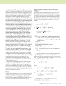
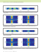
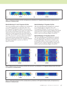
0 5 10 18 18 16 16 14 14 12 12 10 Half skip 5.88 μs Full skip 6.5 μs 8 1.5 4 3.5 3 2.5 2 1.5 1 0.5 0 1 0.5 0 –0.5 –1 –1.5 8 15 x (mm) Time (μs) 20 25 30 1 1 1 110 3 2 1 0 5 m) 0 30 Figure 6. SA-FDTD results of angle-beam UT inspection of two side-drilled holes in a polymer matrix composite: (a) B-scan image (b) A-scan waveform from location marked in B-scan by the dotted line. (a) (b) 5.13 μs 5.38 μs 5.63 μs 5.75 μs 5.88 μs—half skip 6.00 μs 6.13 μs 6.25 μs 6.38 μs 6.50 μs—full skip Figure 7. SA-FDTD wave maps from location noted in Figure 6, showing the UT wave propagation behavior with SDH2 at several discrete time steps: (a) 5.13 μs (b) 5.38 μs (c) 5.63 μs (d) 5.75 μs (e) 5.88 μs (half skip) (f) 6.00 μs (g) 6.13 μs (h) 6.25 μs (i) 6.38 μs (j) 6.50 μs (full skip). The SDH is 0.955 mm in diameter for scale. (a) (d) (c) (b) (e) (f) (g) (h) (i) (j) J A N U A R Y 2 0 2 0 • M A T E R I A L S E V A L U A T I O N 87 Amplitude (a.u.) A (a ) Time (μs) Amplitude (a.u.)
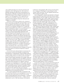
ASNT grants non-exclusive, non-transferable license of this material to  .
All rights reserved. © ASNT 2026. To report unauthorized use, contact: customersupport@asnt.org