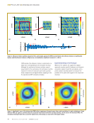
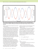
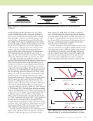
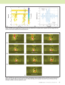
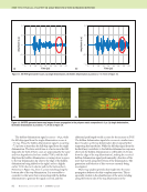
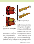
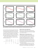
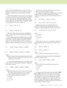
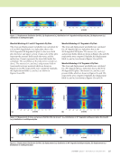
76 M A T E R I A L S E V A L U A T I O N • J A N U A R Y 2 0 2 0 impedance and liftoff variations with probe rotation cannot be excluded at this time. The preceding analysis has shown that the effect of carbon fiber orientation on the response of an eddy current probe can be accurately simulated and that eddy current evaluation can effectively determine the primary fiber orientation directions of a CFRP part. As shown in previous research (Wincheski et al. 2016 Wincheski and Zhao 2018), the technique shown here works well with thicker and more generic fiber layups along with composites containing mismated ply angles. It is anticipated that details of the fiber stacking sequence, fiber areal density, waviness, and embedded damage can also be deduced from a detailed analysis of the probe impedance. In the following section, a voxel-based technique to invert eddy current data to the discretized conductivity tensor throughout the volume of the composite is presented. Voxel-Based, Set-Theoretic Inversion By “voxel-based” we mean that each voxel in the grid of the anomalous region is to be reconstructed in order to determine the anomaly, rather than to model the anomaly at the outset as a canonical structure that is defined by a few parameters that are to be reconstructed. In this sense, voxel-based algorithms are an attempt to eliminate the “curse of dimensionality” malady. The set-theoretic algorithm reconstructs each voxel independently of the other (after a first stage of linear data processing) for example, it is non-Markovian, and yields estimation-quality metrics of each voxel as well. This algorithm is well suited to the volume-integral approach that is the basis of the software used for the computations (Sabbagh et al. 2013). Data are taken using a T/R array, in which each element can be independently used as a transmitter or receiver, as in a “full-matrix capture.” The result of each scan is a “feasible outcome” to an “experiment,” and the set of all possible outcomes is a “feasibility set” for each cell (Combettes 1993). Thus, the data taking is akin to a Monte Carlo test, but in hardware, not software. Feasibility sets are then processed using robust estimators (Sabbagh et al. 2013), to produce outcomes for each cell of the grid. We write the data equation and the field equation as (1) (2) where Z is the coil impedance, E(i) is the incident electric field moment of the klmth-cell due to the probe, J is the electric current at the klmth-cell, E is the total electric field moment in the klmth-cell, and G (ee) is an “electric-electric” Green’s dyadic, which transforms an electric current into an electric field moment. ( ( = [ L †) × †) ( Z(†) E JKLM KLM i) KLM ( ( ) ( ( †) = † [ x [ [ •) × †) ( ( G k K l L E E JKLM , klm i) klm KLM mM ee) ME TECHNICAL PAPER w eddy current characterization for cfrp composites 0 50 100 150 200 250 300 3503 Angle 0 0.1 0.2 0.3 0.4 0.5 0.6 0.7 0.8 0.9 1 0 0.22 0.44 0.66 0.88 1 1.22 1.44 1.66 1.88 2 0 1 1 0 2 0 3 Angle (d(degrees))reeseg 1 2 3 0 4 5 0 6 7 8 0 9 0 0 0 1 1 ΔR sim Δ X sim ΔH exp ΔV exp Figure 4. Simulation and experimental data acquired for 0/90/90/0 composite ply layup. Rsim and Xsim are the calculated change in resistance and reactance while ΔHexp and ΔVexp are the experimentally measured eddy current responses. As explained in the text, the eddy current equipment was configured to nominally align the horizontal and vertical output voltages with changes in resistance and reactance, respectively. Experimental data (volts) Ex p ) Simulation data (ohms)

J A N U A R Y 2 0 2 0 • M A T E R I A L S E V A L U A T I O N 77 The sum is over all cells of the grid. Note that Equations 1 and 2 are linear in all the variables. (See Sabbagh et al. 2013, section 4.2, for further details of the discretization of the volume-integral equation using the electric field moment.) We define the uth “experiment” to be the pair (Z(u), E(i)klm(u)), and the “outcomes” of this experiment to be the pair ( Jklm(u), Eklm(u)), which satisfy Equations 1 and 2. Thus, the outcomes are feasible because they satisfy all known information about the problem. Clearly, we cannot talk about a unique solution, because the feasible set contains many points. Modeling T/R Arrays for Data Taking Each transmitting coil position defines a single experiment or view. For each view, u, we model a single transmitting coil to excite the system and a single receiver coil that is scanned over the region of interest. In place of a single, movable receiver coil, it is possible to use a fixed array of receivers. In either case, this is an example of a T/R configuration, which is becoming more widely used in the NDE industry. The use of a T/R configuration allows us to gain more information from each experiment (that is, from each viewing). For example, if we have a single excitation source (the transmitter), and a single receiver sensor that is scanned over Ns points, then each view, u, produces Ns results, {Z1(u), . . . , ZNs (u)}. The actual current JKLM(u), however, is associated only with the transmitter, because the transmitter is the sole exciter of the system (the receiver is assumed to carry no current). Hence, Equation 1 is replaced by (3) where EKLM (n) (u) is the “incident” field moment produced by the sensor when it is in its nth scan position, during the uth view. In Equations 1 and 3, the expressions for Z are normalized to a driving current of one ampere. This field is known a priori, because we know the location and geometry of the receiving sensor during the uth view. In the model problems to be demonstrated later in this paper, we assume that the host is isotropic and that the receiver coils are oriented in a “pancake” manner. This means that the z-component of the incident field of the receiver coil is zero, which, in turn, means that the z-component of the anomalous current, Jz, makes no contribution to the impedances in the data (Equation 3), and the equation therefore gives us no information about this component. This component is known to be small for the type of receiver coil used. We therefore assume Jz = 0 in our analysis. We also assume that Jx = Jy = 0 for the bottommost of the four layers of our test region. The minimum-norm solution of Equation 3 is given by (4) where M † (u) is the pseudoinverse of the matrix in Equation 3. The electric field moment produced by this current is calculated by substituting Equation 4 into Equation 2: (5) Given the electric field moments, we can then calculate an expansion for the electric field within the discontinuity. The resulting electric field expansion coefficients will be called ˜ klm . Hence, for this value of the view-index, u, we associate the triple, (˜x, ˜x)klm(u), (˜y, ˜y)klm(u), (˜z, ˜z)klm(u), with the klmth cell, and when we take the ratio of the electric current to the electric field at the middle of the klmth cell, we arrive at the conductivity, sklm of the klmth cell, which is the final goal. We then perform another experiment by choosing another value of u, thereby generating another triplet. This ensemble of triplets constitutes the feasible set for each cell. Microstructure Characterization in Carbon Fiber Composites Now we want to apply the previous model to the question of eddy current characterization of carbon fiber composites. The test case is designed to include not only characterization of ply orientation through the thickness of the part, but also fiber areal weight (FAWT) and impact damage. While ply orienta- tion and impact damage are relatively easy to visualize, FAWT and its impact on eddy current measurements may require some introductory discussion. FAWT, measured in grams per square meter, is a way of expressing the fiber density for a given material thickness. By “fiber density” we mean a number between zero and one that indicates how densely distributed the fibers are in the material. If we know the specific gravity of the fiber material and the thickness of the material, we can convert FAWT to fiber density and vice versa. The conversion between fiber density and FAWT may not be a simple task we must take into account the resin content. Increasing the resin content is likely to increase the thickness of the material for a given FAWT, which will probably decrease the fiber density. The thickness of the material is not easily measured. Since the material is made up of many distributed fibers, the thickness at any spot is a random variable, and also depends on how much pressure is applied to the layer. It is not immediately clear exactly how changing FAWT changes the conductivity. We can make a few reasonable assumptions. First, we note that if the FAWT reaches zero, ( ( ( ( ( ( ( ( ( †) = [ x †) × †) †) = [ x †) × †) †) = [ x †) × †) ( ( ( ) Z Z2 Z E J E JKLM E J KLM KLM KLM KLM KLM N KLM KLM N KLM 1 1) 2) s s D ! KLM &) ( = M† &)# ( 1 &) ( s &)! ( %Z $ZN # # " % % ( ( ( ( †) = †) + x [ [ •) × †) ( ( G k K l L Eklm , klm i) KLM mM ee) KLM